LightGBM vs XGBoost vs Catboost

Deep dive into similarities and differences of LightGBM, XGBoost and CatBoost in 10 minutes!

Data Science Letter

Nov 07, 2024

Quick summary

Hello 👋 In this article, I will compare LightGBM, XGBoost and CatBoost in the following areas:

Boosting algorithm
Node splitting
Missing data handling
Feature handling
Data sampling
LightGBM-specific features
XGBoost-specific features
CatBoost-specific features
Tips for choosing between LightGBM, XGBoost and CatBoost
Resources

🚀 Email us @ social@verticalsolution.io if you want us to deep dive into a data science topic!

Boosting algorithm

Conventional boosting (LightGBM, XGBoost) vs Order boosting (CatBoost)

One of the major differences in tree building between LightGBM/XGBoost and CatBoost is the usage of ‘Order boosting’ in CatBoost.

In conventional boosting algorithms (used by LightGBM and XGBoost), at each boosting iteration, the tree is built using the same data points. It is argued that this repeated use of a single set of data points and can increase the chance of overfitting.

To mitigate this effect, CatBoost supports a different boosting algorithm as known as order boosting. The whole idea of this algorithm is to avoid repeatedly using same data points for both tree building and gradient or hessian computations. The method is briefly explained as follows:

First the original training dataset with size N is shuffled S times.
At each boosting iteration, for each shuffled dataset, a separate tree is built for each data position i (where i = 1, 2 ,…, N), using only data points before i (j < i).
The gradients and hessians for a particular data point k are then computed using trees built before k.

In reality, it is not practical to train a tree for each data position for each shuffled datasets, as the computational complexity would scale as SN². The actual algorithm builds trees for a fixed number of data positions K, reducing the complexity to SNK (usually K << N, one example could be K = logN).

In addition, by default CatBoost only performs order boosting when the input dataset size is small. For large datasets, CatBoost will use regular boosting algorithm instead.

Tree growing

Tree growing with LightGBM

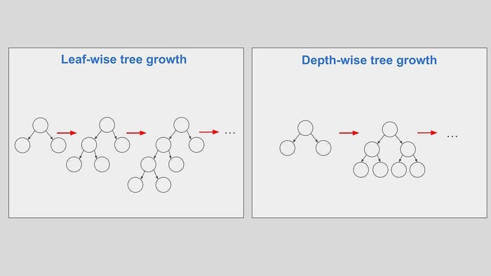
LightGBM: leaf-wise / lossguide

In terms of tree growing methods, LightGBM uses leaf-wise tree growth (also called lossguide in other implementation). In this case, a tree is built leaf by leaf until a maximum number of leaves is attained. In each node splitting iteration, a non-terminal leaf with the best loss improvement is split.

Tree growing with XGBoost

XGBoost: depth-wise / lossguide

XGBoost supports both leaf-wise and depth-wise tree growth, called lossguide and depthwise respectively. In this case, a tree is built level by level until a specific depth is reached. Non-terminal leaves from the previous tree level are split according to each best loss improvement.

Tree growing with CatBoost

CatBoost: symmetric tree, depth-wise / lossguide

CatBoost supports three options: symmetric tree, depthwise and lossguide. The mode SymmetricTree is slightly different from depthwise. While the mode depthwise splits each node with its respective best loss improvement, SymmetricTree splits all node in the same depth with the same splitting criterion.

Node splitting

Node splitting with LightGBM and XGBoost

At each boosting iteration, boosting algorithm finds the optimal splitting position giving the best loss improvement for each node to grow trees.

In each node splitting, the difference in loss before and after splitting is computed:

The detail between each implementation relies on the definition of the loss function.

LightGBM and XGBoost uses primarily second-order approximations with regularisation for computing splitting gain.

In particular, for LightGBM, the splitting gain is defined as:

For XGBoost, the splitting gain is defined as:

Apart from regularisation, the formula of LightGBM and XGBoost look similar to one and other.

Node splitting with CatBoost

CatBoost supports four types of methods to compute splitting gains.

On the other hand, CatBoost supports four different splitting gain criteria, as known as following:

L2, Cosine, NewtonL2 and NewtonCosine

One point to note is that the option of NewtonL2 is similar to the splitting gain definition in LightGBM and XGBoost. For interested users, please visit this page for more information.

Missing data handling

Missing data with LightGBM and XGBoost

During a node split, LightGBM and XGBoost assign the missing data to whichever direction giving the best split in loss.

LightGBM and XGBoost handle missing data by assigning these data points to whichever direction giving the best split in loss. This allows the model to learn from the patterns of missing data.

This feature is quite useful when data imputation or data filtering based on missing values are difficult to do, for example in situations where there are a lot of missing columns.

There is one thing to be mindful of. If there is no missing data in a column during training, but in inference there are missing data, then LightGBM and XGBoost will assign those data points to their respective default directions. Default directions can vary case-by-case. Visit these two discussions (here and here) on git if you are interested. In any case, in terms of model development, it is desirable to investigate on this train-test discrepancy as this can lead to significant degraded model performance from distribution drift.

Missing data with CatBoost

CatBoost either assigns all missing data to the left, or the right, or forbids the presence of missing data.

CatBoost does not provide an adaptive missing data handling as LightGBM or XGBoost. For numerical features, the following modes are supported:

Forbidden — missing data is treated as an error
Min — missing data for a feature is treated as the minimum value for that feature during a node split
Max — missing data for a feature is treated as the maximum value for that feature during a node split

In general, one has to perform more manuel to handle missing data when using CatBoost.

Categorical Feature handling

Categorical features handling with LightGBM

LightGBM supports partitioning of categorical features.

LightGBM handles categorical features by partitioning its categories into 2 subsets and choose the subset which gives the best split, as shown in the figure below:

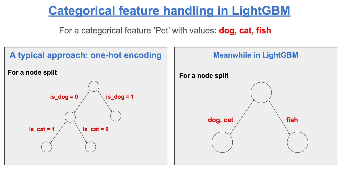
One advantage is that a tree will not need to grow very deep to achieve similar accuracy.

Categorical features handling with XGBoost

XGBoost supports partitioning of categorical features or one-hot encoding.

Starting from version 1.5, XGBoost supports both one-hot encoding and partitioning.

Categorical features handling with CatBoost

CatBoost transforms categorical features to numerical features by order target encoding.

One of the major differences between CatBoost and other boosting algorithm implementations is the way CatBoost handles categorical features.

Order target encoding — One major feature of CatBoost is to allow order target encoding. Normally, target encoding for categorical features can easily lead to data leakage as training labels are directly used as features. Instead, to reduce the risk of data leakage, CatBoost uses the same trick from order boosting datasets to compute target-encoded values for each data point.

For example, for binary classification problems, given a categorical feature with value as A, B, C, one example of the target-encoded value for A is:

where countInA is the sum of binary target with class A in the dataset, and totalCount is the total count of the dataset.

Data sampling

At each boosting iteration, it is possible to select only a fraction of the training datasets to grow the tree. There are a lot of ways to sample datasets. Examples include:

🔴 Uniform sampling means that each data point is independently sampled with a certain probability (a configurable parameter). For example, an uniform sampling of probability 0.3 will mean that at each iteration, roughly 30% of the training data will be used.

🔴 Parametric sampling refers to sampling methods with sampling weights defined by a parametric function, such as exponential or poisson functions.

🔴 Gradient-based sampling refers to sampling methods with sampling weights defined by gradients. The advantage is that data points with smaller gradient are in general well-trained, and hence should be downsampled. This can improve the training speed of the algorithm as some data points are dropped.

LightGBM, XGBoost and CatBoost supports different set of sampling methods. They will be explained below. Let’s start with LightGBM.

Data sampling method in LightGBM

LightGBM supports uniform sampling and a gradient-based sampling method called GOSS.

In LightGBM, the parameter to select sampling strategies is called data_sample_strategy. There are two options:

bagging
goss

Bagging refers to uniform sampling, with probability set by the parameter bagging_fraction.

Another option is called goss, which stands for gradient-based one-side sampling. In this method, top a% of data with the largest gradient values are kept, the remaining (1-a)% of data is downsampled. To avoid drift from original data distribution, the downsampled data are up-weighted in later process. This method ensures that we put more focus on the under-trained samples as the boosting iterations continue.

Data sampling method in XGBoost

XGBoost supports uniform sampling and a gradient-based sampling method.

In XGBoost, the parameter to select sampling strategies is called sampling_method. There are two options:

uniform
gradient_based

With the option uniform, one can set the probability with the parameter subsample.

The gradient-based sampling method supported by XGBoost samples data points according to the weight

where g and h are the gradient and hessian respectively, and lambda is the regularisation parameter. Note that this is a different gradient-based sampling method than the one supported by LightGBM above.

Data sampling method in CatBoost

CatBoost supports four types of sampling strategies: Bernoulli, Bayesian, Poisson and MVS.

In Catboost, the parameter to select sampling strategies is called bootstrap_type. There are four options:

Bayesian
Bernoulli
MVS
Poisson

Despite the difference in name, the Bernoulli sampling method is actually uniform sampling. One can control the probability of sampling with the parameter subsample.

The Bayesian sampling method samples data points with weights defined as:

where w is the weight for each data point. The parameter t is defined the bagging_temperature parameter. This is in fact the Bayesian Bootstrap method proposed by D. Rubin in 1981.

The poisson sampling method samples data points with weights defined as:

Finally, the MVS (Minimum Variance Sampling) method is a gradient-based sampling method. MVS is in some ways similar to GOSS in LightGBM. The differences between this method and the one in LightGBM are:

A threshold is determined on the fly to determine above what values gradients are considered to be large, while in LightGBM a fixed percentage are pre-determined before training.
Data samples with small gradients are weighted with a constant factor in LightGBM, while with MVS they are weighted with a factor proportional to the gradient value.

On theoretical basis, MVS usually gives a lower variance than GOSS. For interested readers, feel free to visit this paper for more detail.

LightGBM-specific features

Pairwise linear regression

Instead of using aggregated statistics, e.g. mean, median, in each leaf for predictions, LightGBM can perform linear regressions within each leaf and use these linear model to generate predictions instead. This function can be enabled by the argument linear_tree. This feature has been implemented since Dec 2020 (see the merge request here)

Exclusive feature bundling

This method aims to reduce the number of sparse features during tree growing by regrouping mutually exclusive sparse features into bundles. This feature aims to reduce memory usage and processing speed of the algorithm. Please refer to the original paper for more detail.

XGBoost-specific features

Survival-analysis

XGBoost supports custom loss functions for various survival analysis. One key difference between ordinary regression and survival analysis is that target labels in survival analysis can be are often represented by a range instead of point estimates, as the upper limit of the survival time can be infinite if the event has not occurred yet. Below shows an example of how to use define and use survival-analysis-specific loss functions in XGBoost.

import numpy as np
import os
import pandas as pd
from sklearn.model_selection import ShuffleSplit

import xgboost as xgb

# Read data
df = pd.read_csv('data.csv')
y_lower_bound = df['y_lower_bound']
y_upper_bound = df['y_upper_bound']
X = df.drop(['y_lower_bound', 'y_upper_bound'], axis=1)

# Train test split
rs = ShuffleSplit(n_splits=2, test_size=.7, random_state=0)
train_index, valid_index = next(rs.split(X))

# Construct train dataset
dtrain = xgb.DMatrix(X.values[train_index, :])
dtrain.set_float_info('y_lower_bound', y_lower_bound[train_index])
dtrain.set_float_info('y_upper_bound', y_upper_bound[train_index])

# Construct valid dataset
dvalid = xgb.DMatrix(X.values[valid_index, :])
dvalid.set_float_info('y_lower_bound', y_lower_bound[valid_index])
dvalid.set_float_info('y_upper_bound', y_upper_bound[valid_index])

# Perform training
params = {
  'verbosity': 0,
  'objective': 'survival:aft',
  'eval_metric': 'aft-nloglik',
  'aft_loss_distribution': 'normal',
  'aft_loss_distribution_scale': 1.20,
  'tree_method': 'hist',
  'learning_rate': 0.01,
  'max_depth': 6,
  'lambda': 0.01,
  'alpha': 0.02
}
bst = xgb.train(
  params, dtrain, 
  num_boost_round=10000,
  evals=[(dtrain, 'train'), (dvalid, 'valid')],
  early_stopping_rounds=50,
)

How to choose between LightGBM, XGBoost and CatBoost

Here are a few aspects to be considered when choosing between LightGBM, XGBoost, and CatBoost:

Memory storage and processing speed

LightGBM is in general a faster implementation among the three. If memory storage or training speed is a concern (e.g. when you have a dataframe using a large fraction of your memory already), it is probably good to try first LightGBM.

Missing data handling

LightGBM and XGBoost can assign data points with missing values that best optimise the objective function, while CatBoost does not support this feature. If your dataset has a lot of missing values and you would like to let the algorithm figure out its dependency by itself, it is probably best to use LightGBM and XGBoost.

Both LightGBM and XGBoost uses partitioning by default so it is not needed to do anything before training. (Note that this method only works for missing values in feature columns. In general it does not make sense to have missing values in target columns)

Overfitting

Regularisation parameters between the three implementations are more or less similar. In each implementation, there are a few common parameters that we can use to regularise the training and control overfitting, here are a few examples:

Number of leaves ➡️ Maximum number of leaves in each tree (The higher this number, the more complex the trees will become)
Maximum depth ➡️ Maximum number of depth in each tree (The higher this number, the more complex the trees will become)
Data sampling fraction ➡️ The fraction of training data to be used in each boosting iteration. This reduces the likelihood of having a small portion of the training data dominating the training process and leads to overfitting
Data sampling frequency ➡️ The frequency of which the training data will be sampled
Feature fraction ➡️ The fraction of training data to be used in each boosting iteration
Early stopping ➡️ Stop training whenever the performance does not improve for a while
Lambda L1 or L2 ➡️ These few regularisation control the complexity of the trees (The higher these numbers, the less complex the trees are)
dropout rate for DART (LightGBM or XGBoost) ➡️ During training, a fraction of trained trees are dropped at a certain probability. This helps regularise the whole algorithm as this removes over-dependency on a few trees.

For relatively small datasets with which overfitting is often a problem, one can consider to use order boosting in CatBoost.

Categorical feature handling

Both LightGBM and XGBoost support the functionalities to use one-hot encoding or partitioning for categorical features during node splitting, while CatBoost relies on order target encoding.

Target encoding works better when target labels have strong correlations with encoding categories. The disadvantage is that this technique is in general more prone to overfitting.

Linear model

Both LightGBM and XGBoost support linear models for predictions, instead of simple aggregated statistics, such as mean of target labels, from the leaves. This gives more flexibility for model developments.